RoPE: Rotary Position Embeddings Explained

Hello readers, in our previous blogs, we learned about Positional Embeddings and Self Attention. Today, we will learn about another type of positional embedding, i.e. RoPE, and why it is needed.

A Brief Recap#

Just to give a brief recap:

Positional Embeddings#

We learned about sinusoidal embeddings and how they preserve positional information while keeping their magnitude bounded. We were “adding” this positional data to our existing token embeddings to make them position-aware.

$$\text{Embeddings} = \text{Token Embeddings} + \text{Positional Embeddings}$$

Self Attention#

We compute “query”, “key” and “value” projections for a given embedding. Then we compute the attention score using:

The Issue with the Current Approach#

While computing attention scores, we do a matrix multiplication of the query and key matrices.

A matrix multiplication is similar to taking a dot product from the point of view of each row. How?

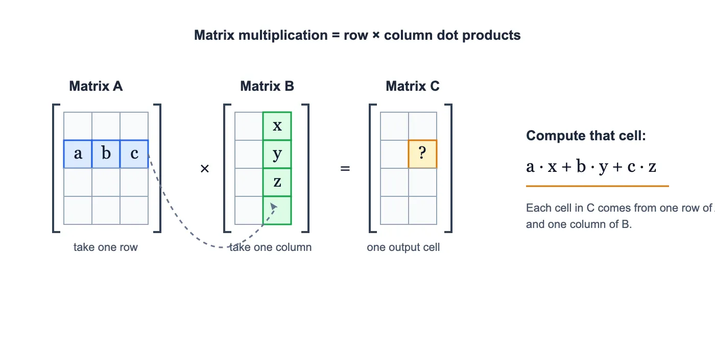
So, with our current embedding approach:

E = T + P

where E -> Embedding
      T -> Token Embedding
      P -> Positional Embedding

While computing the Query and Key projections, we can denote them as:

Q = Q(T + P)
K = K(T + P)

Now, while computing attention scores, we take the dot product of Q and K. Let’s consider there are 2 positions ‘x’ and ‘y’, and we are computing the attention score between them:

Score = Qx . Ky
      = Q(Tx + Px) . K(Ty + Py)
      = S[(Tx + Px) . (Ty + Py)]
      = S[TxTy + TxPy + PxTy + PxPy]

If we look carefully at each by-product:

• TxTy captures the token data
• PxPy captures the positional data
• But the remaining 2 by-products, i.e. (TxPy and PxTy), are garbage — they don’t denote anything

Now, this garbage data is eventually supplied to our neural network, and it has to make some meaning out of it. And as you know, there are multiple attention blocks and not just one, so the issue cascades into a major degradation.

Intuition#

If you notice, up until now our approach was to “add” positional data to our token embeddings, and this “addition” was the root cause of our garbage by-products.

What if, instead of an “addition”, we do a “rotation”?

E = T(θ)

where θ (theta) is the angle

So the attention score becomes:

Score = Q(T(θ1)x) . K(T(θ2)y)

Using the dot product formula:

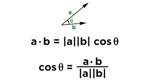
Score = |Tx| |Ty| Cos(θ1 - θ2)

If you notice, the score now brings together the token magnitudes and the difference between the rotation angles.

Implementation#

Now that we have built the intuition, let’s see how we can fit it into our current design.

Split the Dimensions into Pairs#

Up until now, we had token embeddings of “n” dimensions. To work with rotations, let’s group those dimensions into 2D planes.

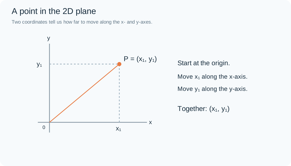
To represent a point in a 2D plane, we need two coordinates, i.e., $(x, y)$.

So, we will split our n-dimensional embedding into pairs of two, such that each pair represents a point in its own 2D plane. Here, we assume that n is even.

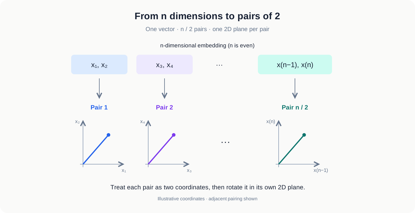
Now, for our n-dimensional embedding, we have $n/2$ pairs that we can rotate to store positional information.

Assign a Rotation to Each Pair#

Let’s use $d = n$ for the number of dimensions in the frequency formula. For a token at position p, the rotation angles are:

$$P(p) = [\phi_0(p), \phi_1(p), \ldots, \phi_{d/2-1}(p)]$$ $$\omega_i = 10000^{-2i/d}, \qquad \phi_i(p) = p\,\omega_i, \qquad i = 0,1,\ldots,\frac{d}{2}-1$$

Here, $\omega_i$ is the frequency of pair i, and $\phi_i(p)$ is its rotation angle at position p. So, each pair rotates at its own frequency as we move through the sequence.

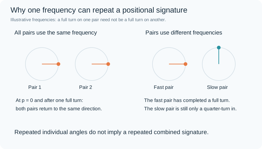
You might be wondering why we don’t use the same frequency for every pair.

Well, a rotation repeats after a full turn. If all pairs use the same frequency, they return to their starting directions together. Using different frequencies helps distinguish positions by looking at the combined signature across all pairs.

Understand the Rotation#

So, now we have a way to represent positions through rotations. How do we apply those rotations to our embedding pairs? For that, let’s first understand the rotation matrix.

In a typical 2D plane, let’s say we have a point $(x_1, y_1)$.

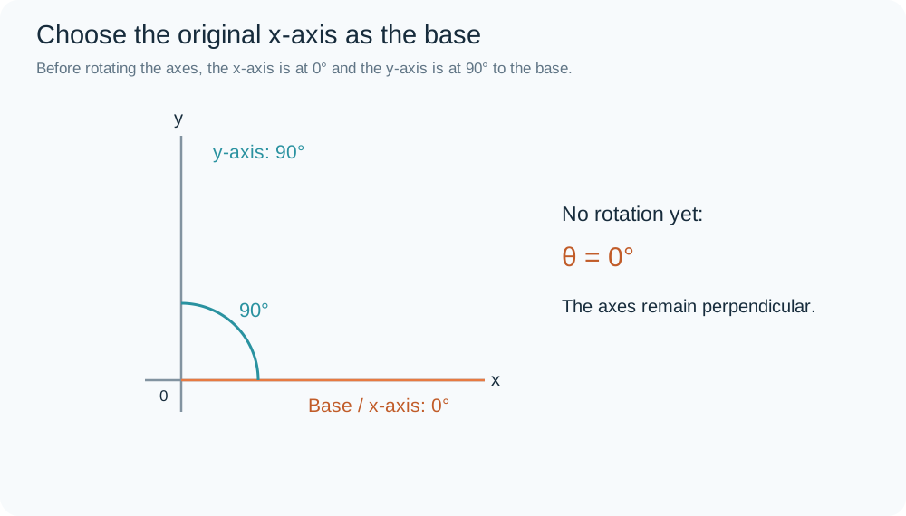
Let’s take our current x-axis as the “base.” Before any rotation, the x-axis makes an angle of 0° with this base, while the y-axis makes an angle of 90°.

We will use $\theta$ to denote how far we rotate the reference axes from their original orientation.

Up until now, we represented our point using its coordinates along the original axes. Now, let’s express the same point relative to axes rotated by an angle $\theta$.

The new coordinates are:

$$\begin{aligned} x_1' &= x_1\cos\theta + y_1\sin\theta \\ y_1' &= -x_1\sin\theta + y_1\cos\theta \end{aligned}$$

Let’s first check the “normal” scenario, where $\theta = 0$:

$$\begin{aligned} x_1' &= x_1\cos 0 + y_1\sin 0 = x_1 \\ y_1' &= -x_1\sin 0 + y_1\cos 0 = y_1 \end{aligned}$$

As expected, when we don’t rotate the axes, the coordinates stay the same.

But if we rotate the x- and y-axes counterclockwise by $\theta$, the same point gets a new pair of coordinates relative to those axes:

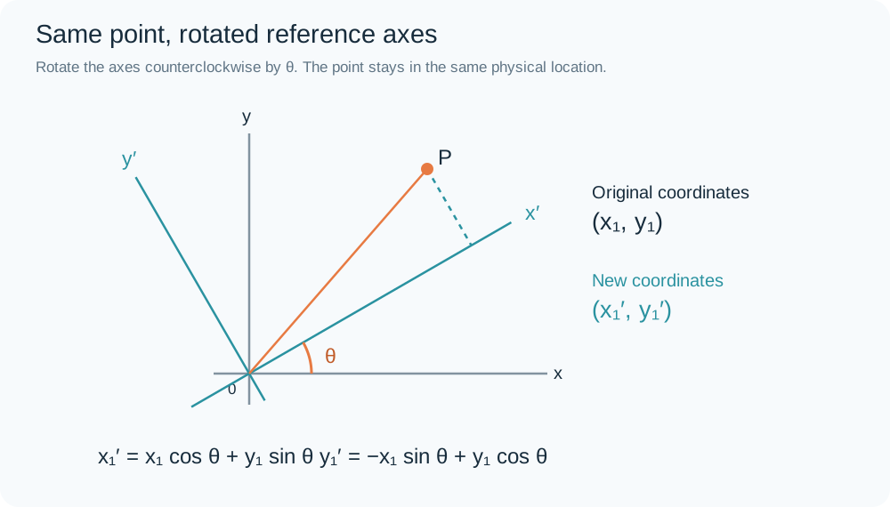
Note: In this explanation, we are rotating the reference axes while keeping the point fixed. This is the convention used by the signs in the equations above.

Write It as a Matrix#

So, now we have the intuition behind the coordinate transformation. You might be wondering why we keep calling it a “rotation matrix” when we haven’t used a matrix yet.

Well, if you look carefully, those two equations can be written together as:

$$\begin{bmatrix} x_1'\\ y_1' \end{bmatrix} = \underbrace{ \begin{bmatrix} \cos\theta & \sin\theta\\ -\sin\theta & \cos\theta \end{bmatrix} }_{R(\theta)} \begin{bmatrix} x_1\\ y_1 \end{bmatrix}$$

Here, $R(\theta)$ is our rotation matrix. Multiplying it by the coordinate pair gives us the same two equations we just worked through.

Put the Pairs Together#

Now, let’s stitch everything together.

Our embedding pairs were:

$$[(x_1,x_2),\ (x_3,x_4),\ \ldots,\ (x_{n-1},x_n)]$$

Each pair has its own angle, so its own rotation matrix:

$$R(\phi_0(p)),\ R(\phi_1(p)),\ \ldots,\ R(\phi_{n/2-1}(p))$$

We can combine them into one larger matrix by placing the 2 × 2 rotation matrices along the diagonal and filling the remaining entries with zeros:

$$R_p = \begin{bmatrix} c_0 & s_0 & 0 & 0 & \cdots & 0 & 0\\ -s_0 & c_0 & 0 & 0 & \cdots & 0 & 0\\ 0 & 0 & c_1 & s_1 & \cdots & 0 & 0\\ 0 & 0 & -s_1 & c_1 & \cdots & 0 & 0\\ \vdots & \vdots & \vdots & \vdots & \ddots & \vdots & \vdots\\ 0 & 0 & 0 & 0 & \cdots & c_{n/2-1} & s_{n/2-1}\\ 0 & 0 & 0 & 0 & \cdots & -s_{n/2-1} & c_{n/2-1} \end{bmatrix}$$

where:

$$c_i = \cos(\phi_i(p)), \qquad s_i = \sin(\phi_i(p))$$

Using column vectors, the complete transformation is:

$$\underbrace{ \begin{bmatrix} x_1'\\x_2'\\\vdots\\x_{n-1}'\\x_n' \end{bmatrix} }_{\text{Position-aware embedding}} = R_p \underbrace{ \begin{bmatrix} x_1\\x_2\\\vdots\\x_{n-1}\\x_n \end{bmatrix} }_{\text{Embedding}}$$

If we write embeddings as row vectors instead, the same transformation is:

$$\mathbf{x}'_{\mathrm{row}} = \mathbf{x}_{\mathrm{row}}R_p^{\mathsf T}$$

So, each pair rotates by its assigned angle, and all the rotated pairs come together to form our position-aware representation.

RoPE Scaling#

There is one more interesting idea that comes out of these rotations: RoPE scaling. Let’s see what that means.

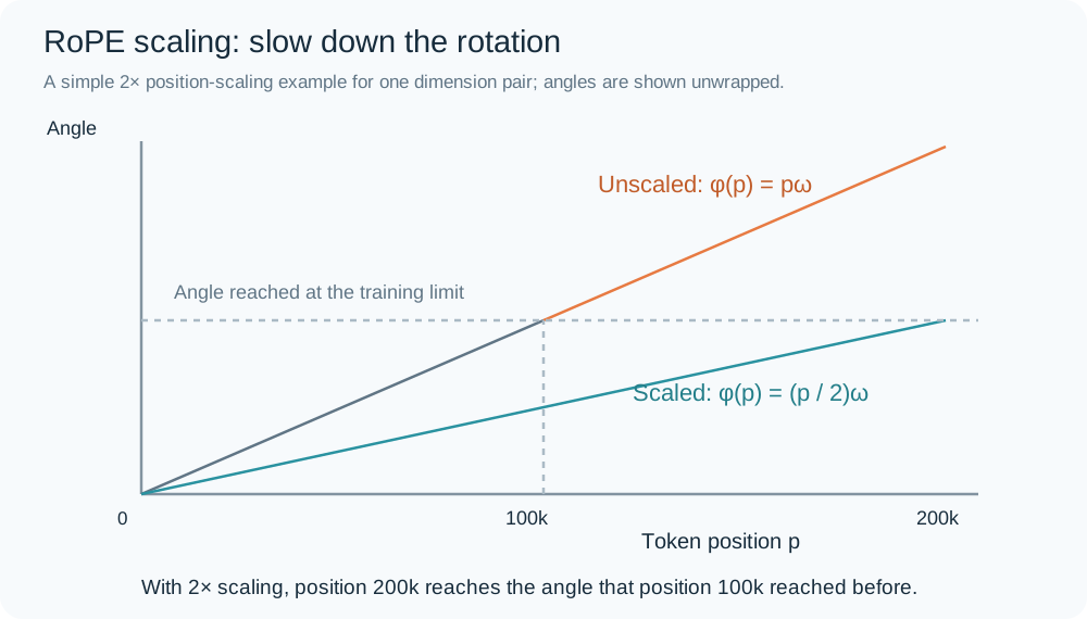
Let’s say we have a model trained on a context length of 100k tokens. If we supply 200k tokens, we cannot simply expect it to behave the same way. The larger positions take its rotations beyond the position range it encountered during training.

That’s where RoPE scaling comes into play. The basic idea is to slow down the rotations so that a longer sequence can fit into a more familiar range of rotation angles.

For a simple 2× scaling example, we can write:

$$\phi_i^{\text{scaled}}(p) = \frac{p}{2}\,\omega_i$$

At position 200k, the scaled angle now matches the unscaled angle at position 100k.

We can also adjust the base used in the frequency formula:

$$\omega_i = \mathrm{base}^{-2i/d}$$

Here, 10000 was our original base. Changing the base changes the frequencies across the dimension pairs, giving us another way to adjust how quickly they rotate. This is different from dividing every position by the same factor, but the intuition is similar: adjust the rotations for the longer context.

Conclusion#

I hope you now have a clearer picture of what RoPE is and enough intuition that it no longer feels like an unfamiliar concept.

We started with the idea of encoding positions through rotations, split our embedding into pairs, and brought those rotations together using a matrix. We also saw how slowing down the rotations leads to the idea of RoPE scaling.

Thanks for reading, and stay tuned for more…

Further reading#

• Su et al.: RoFormer — Enhanced Transformer with Rotary Position Embedding — the paper that introduced RoPE, with the relative-position property proved in section 3.